Counties

Perspectives on US Counties and how skewed population distributions are

A few large counties contain a large proportion of the US population. This vignette briefly explores the distribution of counties in the US, particularly how many counties have a large number of block groups and residents.

Note there are also guides to using EJAM in R for County/FIPS analysis and reference documents on relevant R functions and county-related test data.

The US has over 3,200 Counties but the 80/20 rule applies almost exactly – About 80% of the population is in just 20% of all Counties. In fact, most of the US population lives in less than 5% of all US Counties. About 150 counties account for most of the US residents.

# code to get stats on population and blockgroup counts by county
z <- blockgroupstats[ , .(pop = sum(pop), bgcount = .N), 
     by = .(countyfips = substr(bgfips,1,5))][order(bgcount), ]
z[ , name := fips2name(countyfips)]
setcolorder(z, "countyfips", after = NCOL(z))
setcolorder(z, "bgcount")
setorder(z, -bgcount)
# percent of residents and percent of counties
zz <- z[order(-pop), ]
zz$cumpop = cumsum(zz$pop)
zz$cumpctpop = round(100 * zz$cumpop / sum(zz$pop),1)
zz[, cumpctcounties := round(100 * .I/NROW(zz), 1) ]
which(zz$cumpctpop >= 50 )[1]
#> [1] 147
zz[cumpctpop >= 50, ][1, .(cumpctpop, cumpctcounties)]
#>    cumpctpop cumpctcounties
#>        <num>          <num>
#> 1:        50            4.6

Map of counties with at least 1 million residents each

# code to show the map of key counties
suppressWarnings({ suppressMessages({
shp1 <- shapes_from_fips(fips = z[pop >= 1e6, ]$countyfips)
shp1 <- cbind(shp1, pop = z[pop >= 1e6, ]$pop)
mapfast(shp1)
})}) 

  ## to see the map of key counties in a web browser:
  # mp <- mapfast(shp1, launch_browser = TRUE)

Histogram showing county population is usually between 10 thousand and 100 thousand, but can be much less or much more fairly often.

hist(log10(z$pop), 1000 , axes=F,
     xlab="Log scale of population count by county",
     main = "Population size varies greatly across US Counties")
axis(side = 1, at = 2:7,
     labels = c(100, '1,000','10 thousand', '100 thousand', 
                "1 million", "10 m")) 

Scatterplot of population and # of blockgroups, by county

plot(z$bgcount, z$pop, 
     xlab = "# of blockgroups in the county",
     ylab = "County population", log =  'xy')

Map of counties with more than 1,000 blockgroups each

shp2 <- cbind(
  shapes_from_fips(fips = z[bgcount >= 1000, ]$countyfips),
  blockgroup_count = z[bgcount >= 1000, ]$bgcount)
suppressMessages(suppressWarnings({
  mapfast(shp2)
  ## to see the map of key counties in a web browser:
  # mp <- mapfast(shp2, launch_browser = TRUE)
}))

A handful of counties have over 1,000 block groups each, while most counties have less than 25 block groups each. These are the largest counties in terms of how many blockgroups they contain:

x = data.frame(z[bgcount >= 1000, ])
x$pop = prettyNum(x$pop, big.mark = ",")
x$bgcount = prettyNum(x$bgcount, big.mark = ",")
print(x)
#>    bgcount       pop                      name countyfips
#> 1    6,591 9,936,690    Los Angeles County, CA      06037
#> 2    4,002 5,225,367           Cook County, IL      17031
#> 3    2,830 4,726,177         Harris County, TX      48201
#> 4    2,806 4,430,871       Maricopa County, AZ      04013
#> 5    2,156 2,679,620          Kings County, NY      36047
#> 6    2,058 3,289,701      San Diego County, CA      06073
#> 7    2,049 3,175,227         Orange County, CA      06059
#> 8    1,843 2,688,237     Miami-Dade County, FL      12086
#> 9    1,803 2,360,826         Queens County, NY      36081
#> 10   1,570 2,604,053         Dallas County, TX      48113
#> 11   1,545 2,254,371           King County, WA      53033
#> 12   1,507 1,781,641          Wayne County, MI      26163
#> 13   1,394 2,429,487      Riverside County, CA      06065
#> 14   1,338 1,593,208   Philadelphia County, PA      42101
#> 15   1,325 2,265,926          Clark County, NV      32003
#> 16   1,292 1,645,867       New York County, NY      36061
#> 17   1,275 2,180,563 San Bernardino County, CA      06071
#> 18   1,246 2,113,854        Tarrant County, TX      48439
#> 19   1,185 1,256,620       Cuyahoga County, OH      39035
#> 20   1,182 1,443,229          Bronx County, NY      36005
#> 21   1,176 1,623,109      Middlesex County, MA      25017
#> 22   1,173 1,916,831    Santa Clara County, CA      06085
#> 23   1,139 1,389,160         Nassau County, NY      36059
#> 24   1,139 2,014,059          Bexar County, TX      48029
#> 25   1,134 1,663,823        Alameda County, CA      06001
#> 26   1,121 1,940,907        Broward County, FL      12011
#> 27   1,098 1,270,787       Hennepin County, MN      27053
#> 28   1,062 1,245,310      Allegheny County, PA      42003
#> 29   1,060 1,272,264        Oakland County, MI      26125
#> 30   1,058 1,524,486        Suffolk County, NY      36103
#> 31   1,024 1,579,211     Sacramento County, CA      06067
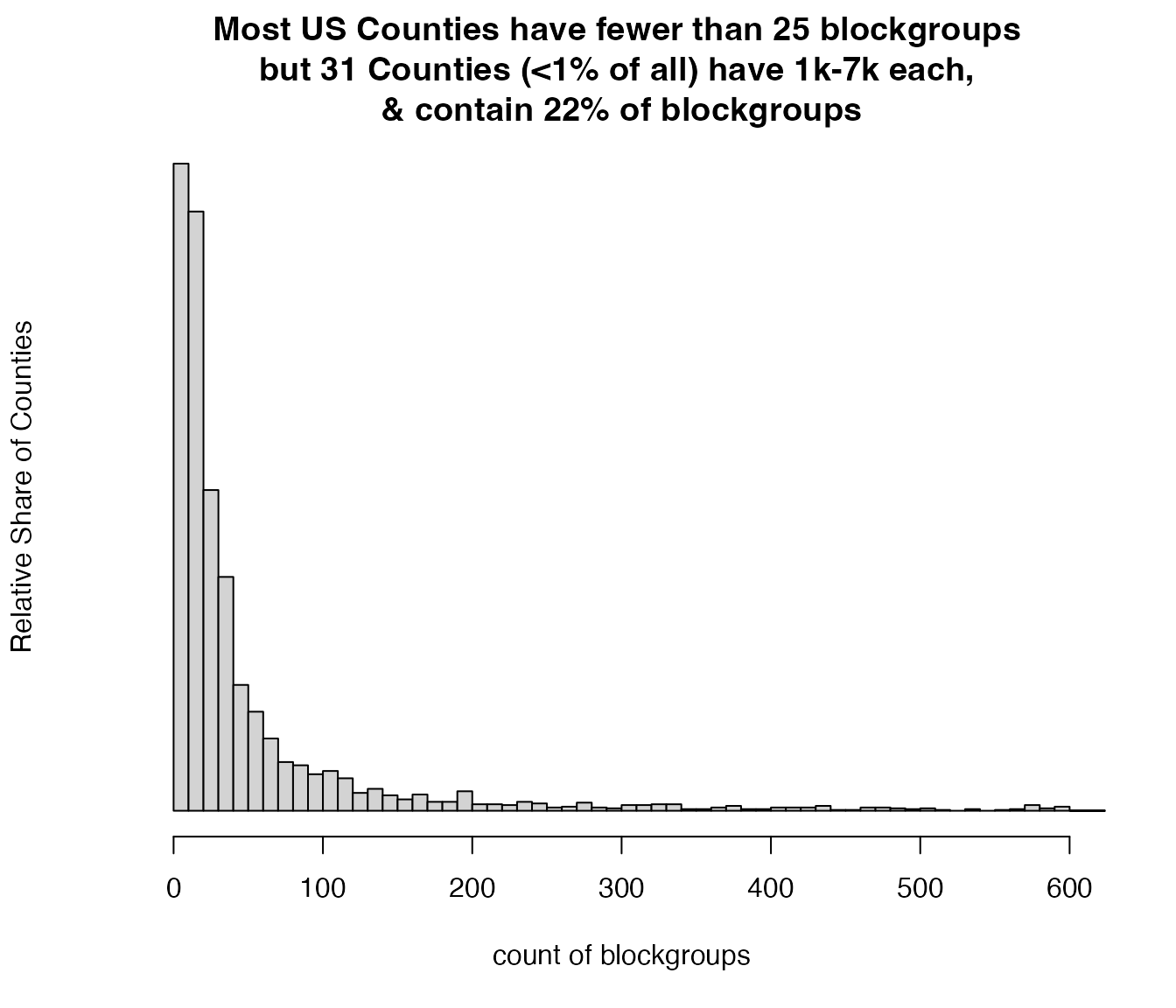
# print( z[bgcount >= 1000, ][] )

Histogram showing that most counties have fewer than 25 blockgroups, but a few have over 1000 each

hist(z$bgcount, breaks = c((0:60)*10,10000), xlim=c(0, 600), 
     main = "Most US Counties have fewer than 25 blockgroups 
but 31 Counties (<1% of all) have 1k-7k each, 
& contain 22% of blockgroups", 
xlab = "count of blockgroups", 
ylab = "Relative Share of Counties", yaxt="n")